Simultaneous Localization and Map Building: Test case for Outdoor Applications 

 

Jose Guivant, Eduardo Nebot

Australian Centre for Field Robotics

Department of Mechanical and Mechatronic Engineering

The University of Sydney, NSW 2006, Australia

jguivant/nebot@acfr.usyd.edu.au

 

 

 

Abstract.  This work presents real-time algorithms and implementation issues of Simultaneous Localization and Map Building (SLAM) with emphasis to outdoor land vehicle applications in large environments. It presents the problematic of outdoors navigation using feature based localization methods. The aspect of feature detection and validation is investigated to reliable detect the predominant features in the environment. The SLAM algorithm presented uses a compressed filter to maintain the map with a cost ~O(N_a²), where N_a is the number of landmarks in the local area. The information gathered in the local area is then transferred to the overall map in one iteration at full SLAM computational cost when the vehicle leaves the local area. Algorithms to simplify the full update are also presented that results in a near optimal solution. Finally the algorithms are validated with experimental results obtained with a standard vehicle running in unstructured outdoor environment. This work uses a series of multimedia facilities to clearly demonstrate the problematic of outdoor navigation in unstructured environments. The results are presented with a series of animations that demonstrates the main features of the algorithm presented. The raw dead-reckoning, laser data and matlab code used to identify the features can also be accessed. This is essential to compare localization and map building results obtained with other localization algorithms.

1          Introduction

The problem of localization given a map of the environment or estimating the map knowing the vehicle position is known to be a solved problem and in fact applied in many research and industrial applications [1,2,3]. A much more complicate problem is when both, the map and the vehicle position are not known. This problem is usually referred as Simultaneous Localization and Map Building (SLAM) [4] / Concurrent Map Building and Localisation (CML) [5].  It has been addressed using different techniques such as in [6] where approximation of the probability density functions with samples is used to represent uncertainty. In this case no assumption needs to be made on the particular model and sensor distributions. The algorithm is suitable to handle multi-modal distribution. Although it has proved robust in many localization applications, due to the high computation requirements this method has not been used for real time SLAM yet, although work is in progress to overcome this limitation. 

Kalman Filter can also be extended to solve the SLAM problem, [7, 8, 9] once appropriate models for the vehicle and sensors are obtained. This method requires the robot to be localised all the time with a certain accuracy. This is not an issue for many industrial applications, [2,3, 10,11], where the navigation system has to be designed with enough integrity in order to avoid/detect degradation of localisation accuracy. For these applications the Kalman Filter with Gaussian assumptions is the preferred approach to achieve the degree of integrity required in such environments.

One of the main problems with the SLAM algorithm has been the computational requirements that is of the order ~O (N²) [12], N being the number of landmarks in the map. In large environments the number of landmarks detected will make the computational requirement to be beyond the power capabilities of the computer resources. The computational issues of SLAM have been addressed with a number of suboptimal simplification, such as [4] and [5]. This paper presents real time implementation of SLAM with a set of optimal algorithms that significantly reduce the computational requirement without introducing any penalties in the accuracy of the results. Sub-optimal simplifications are also implemented to update the covariance matrix of the states when full SLAM is required. The convergence and accuracy of the algorithm are tested in large outdoor environments with more than 500 states.

The paper is organized as follows. Section 2 presents an introduction to the SLAM problem and the vehicle and sensor models used in this applications. Section 3 presents the navigation environment and the algorithms used to detect and validate the most relevant features in the environment. These two sections are essential to compare different algorithms independent of the modelling aspect and the methods used to extract the features from the environment. Section 4 presents a brief description of the compressed algorithm used to implement SLAM. Section 5 presents important implementation issues such as map management and simplifications to perform full update in a sub-optimal manner. Section 6 presents experimental results in unstructured outdoor environments. Finally Section 7 presents conclusions and a presentation of important research issues of autonomous navigation.

2          Simultaneous Localization and Map Building (SLAM)

When absolute position information is not available it is still possible to navigate with small errors for long periods of time. The SLAM algorithm addresses the problem of a vehicle with known kinematic, starting at an unknown position and moving through an unknown environment populated with some type of features. The algorithm uses dead reckoning and relative observation to detect features, to estimate the position of the vehicle and to build and maintain a navigation map as shown in Figure 1. With appropriate planing the vehicle will be able to build a relative map of the environment and localize itself. If the initial position is known with respect to a global reference frame or if absolute position information is received during the navigation task then the map can be registered to the global frame. If not the vehicle can still navigate in the local map performing a given task, explore and incorporate new areas to the map.

 

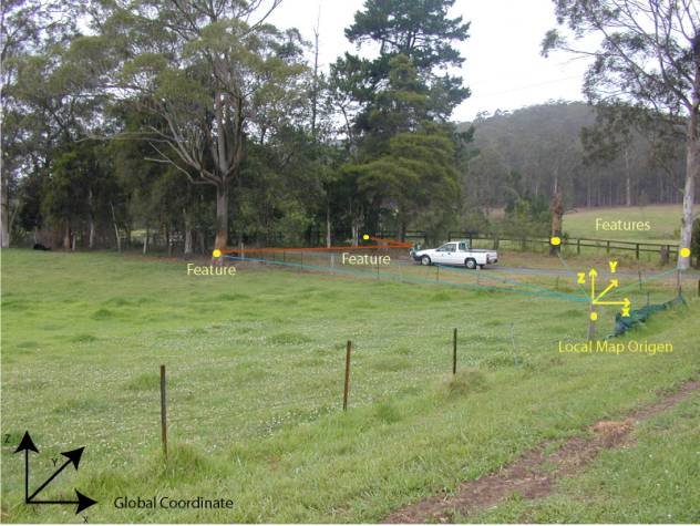
Figure 1. Navigation using SLAM. The vehicle build a relative local map and localise within this map using dead reckoning information and relative observation of the features in the local environment. The accuracy of the map is a function of the accuracy of the local map origen and the quality of the kinematic model and relative observations. The local map can eventually be registered with the global map if absolute information become available, such as the observation of a beacon at a known position or GPS position information.

 

A typical kinematic model of a land vehicle can be obtained from Figure 2 . The steering control a, and the speed u_c are used with the kinematic model to predict the position of the vehicle. The external sensor information is processed to extract features of the environment, in this case called B_i(i=1..n), and to obtain relative range and bearing, , with respect to the vehicle pose.

 

 

Figure 2Vehicle coordinate system

Considering that the vehicle is controlled through a demanded velocity v_c and steering angle athe process model that predicts the trajectory of the centre of the back axle is given by

                                                                                                                    (1)

Where L is the distance between wheel axles and g is white noise. The observation equation relating the vehicle states to the observations is

                                                      (2)

where z is the observation vector,  is the coordinates of the landmarks, x_L, y_L and f_Lare the vehicle states defined at the external sensor location and g_h the sensor noise.

In the case where multiple observation are obtained the observation vector will have the form:

                                                                                                                                              (3)

Under the SLAM framework the vehicle starts at an unknown position with given uncertainty and obtains measurements of the environment relative to its location. This information is used to incrementally build and maintain a navigation map and to localize with respect to this map. The system will detect new features at the beginning of the mission and when the vehicle explores new areas. Once these features become reliable and stable they are incorporated into the map becoming part of the state vector.

The state vector is now given by:

                                                                                           (4)

where (x,y,f)_L and (x,y)_i are the states of the vehicle and features incorporated into the map respectively. Since this environment is consider to be static the dynamic model that includes the new states becomes:

                                                                                                       (5)

It is important to remarks that the landmarks are assumed to be static. Then the Jacobian matrix for the extended system is

                                                                                       (6)

These models can then be used with a standard EKF algorithm to build and maintain a navigation map of the environment and to track the position of the vehicle.

The Prediction stage is required to obtain the predicted value of the states X and its error covariance P at time k based on the information available up to time k-1,

                                                                                      (7)

The update stage is function of the observation model and the error covariances:

                                     (8)

Where

                                        (9)

are the Jacobian matrices derived from vectorial functions F(x,u) and h(x) respect to the state X . R and Q are the error covariance matrices characterizing the noise in the observations and model respectively.

3          Environment Description and Feature detection

The navigation map is built with features present in the environment that can be detected by the external sensor. Recognizable features are essential for SLAM since the algorithm will not operate correctly in a featureless environment.

One of the first tasks in the navigation system design is to determine the type of sensor required to obtain a desired localization accuracy in a particular outdoor environment. The most important factor that determines the quality of the map is obviously the accuracy of the relative external sensor. For example, in the case of radar or laser sensors, this is determined by the range and bearing errors obtained when seeing a feature/landmark. These errors are function of the specification of the sensors and the type of feature used. If the shape of the feature is well known a-priori, such as the case of artificial landmarks, then the errors can be evaluated and the accuracy of the navigation system can be estimated.

A different problem is when the navigation system has to work with natural features. The inspection of the environment can give an idea of the most relevant features that can be detected with a given sensor. The most appropriate sensor for the application will also be a function of the size of the operating area and environmental conditions. Figure 3 presents an outdoor environment where trees can be consider one of the most relevant features that a laser range sensor can identify. This is clearly shown in the video linked to the Figure.  With larger areas or in environment where fog can be present then a different sensor such as radar will be the best choice.

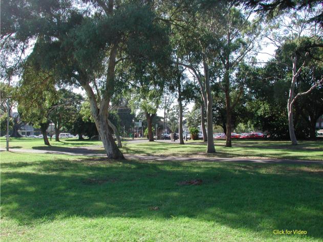
Figure 3Outdoor environment with trees as the most common natural features.  The video presents a complete view of the envirnonment

 

Once the sensor is selected then a model to obtain accurate and consistent position estimation of the features is required. If the raw return from the laser is used as a measure of a distance to a tree then a significant error can be introduced due to the size, shape and inclination of the trunk. This common problem is shown in Figure 4 for various type of trees commonly found in these environments. Each figure has a link to a video that shows the complexity of the problem.  Any algorithm designed to extract the location of these features needs to consider these problems to increase the accuracy of the feature location process. In this work a Kalman Filter was implemented to track the centre of the trunk by clustering a number of laser observations as representative of the circular surface of the trunk.

  

Figure4 Trees with different shape, size and inclination. The feature detection algorithm needs to consider these type of different trees to accurately determine the position of the feature. This problem is shown in the videos linked to each photo

3.1        Feature Position Determination

The landmark’s observations can be improved by evaluating the diameter of the tree trunk considering the most common problems detailed above. This will also make the observation information almost independent of the sensor viewpoint location. The first stage of the process consists of determining the number of consecutive laser returns that belong to the cluster associated to an object, in this case a tree trunk. In the case of working with a range and bearing sensors the information returned from a cylindrical objects is shown in Figure 5 . Depending on the angular and range resolution and beam angle, the sensor will return a number of ranges distributed in a semicircle. In Figure 5 the cylindrical object is detected at four different bearing angles.

Figure 5Laser range finder return information from a cylinder type object

An observation of the Diameter of the feature can be generated using the average range and bearing angle enclosing the cluster of points representing the object:

                                                                                                                                        (10)

Where  are the angular width and average distance to the object obtained from the laser location. For the case of a laser returning 361 range and bearing observations distributed in 180 degrees:

                                                                                             (11)

The indexes i_n to i_i correspond to the first and last beam respectively reflected by the object. The measurement z­_D is obtained from range and bearing information corrupted by noise . The variance of the observation z­_D can then be evaluated:

                                      (12)

In outdoor applications the ranges are in the order of 3-40 metres. In this case we have that:

                                                                                                              (13)

then

                                                                                                                               (14)

This fact indicates that the correlation between z_D and the range measurement error is weak and can be neglected.

Additional noise ws is also included to consider the fact that this type of natural features will be in practice not perfectly circular and will have different diameter at different heights. Depending on the vehicle inclination two scans from the same location could generate a slightly different shape for the same object. The complete model that considers the additional noise ws is:

                                                                                                                (15)

Finally a Kalman filter to track each object is implemented assuming a process model with constant Diameter and initial condition generated with the first observation:

                                                                                                                (16)

The Diameter of each feature is updated after each scan and then used to evaluate the range and bearing to the centre of the trunk. Figure 6presents a set of experimental data points, the circumference correspondent to the estimated Diameter and the centre of the object based on processing the Kalman Filter presented after a few laser frames.

  

Figure 6Tree profile and system approximation. The dots indicate the laser range and bearing returns. The filter estimates the radius of the circumference that approximates the trunk of the tree and centre position.

The video presents the behaviour of the algorithm when tracking different trees. The blue dots correspond to the laser returns and the red circle is the position of the centre of the trunk evaluated by the filter. The matlab program and data files are also provided. These algorithms are essential if different feature based SLAM algorithms are to be compared.

 

4          Real time Implementation of SLAM

In most SLAM applications the number of vehicle states will be insignificant with respect to the number of landmarks. Under the SLAM framework the size of the state vector is equal to the number of the vehicle states plus twice the number of landmarks, that is 2N+3 = M. This is valid when working with point landmarks in 2-D environments. The number of landmarks will grow with the area of operation making the standard filter computation impracticable for on-line applications.

In this work we used the compressed filter algorithm [13] to reduce the real time computation requirement to ~O(2N_a²), being N_a the landmarks in the local area. This will also make the SLAM algorithm extremely efficient while the vehicle remains navigating in this area since the computation complexity becomes independent of the size of the global map.

4.1        Compressed Filter

A common scenario is to have a mobile robot moving in an area and observing features within this area. This situation is shown in Figure 7 where the vehicle is operating in a local area A. The rest of the map is part of the global area B. 

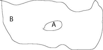
Figure 7Local and Global areas

Consider the states divided in 2 groups

The states X_A can be initially selected as all the states representing features in an area of a certain size surrounding the vehicle. The states representing the vehicle pose are also included in X_A.   Assume that for a period of time the observations obtained are only related with the states X_A and do not involve states of X_B, that is 

                                                                                                                                (17)

Then at a given time k

                            (18)

Considering the zeros of the matrix H the Kalman gain matrix W is evaluated as follows

                                                                          (19)

From these equations it is possible to see that

1.      The Jacobian matrix H_a has no dependence on the states X_B.

2.      The innovation covariance matrix S and Kalman gain W_a are function of P_aa and H_a. They do not have any dependence on P_bb, P_ab, P_ba and X_b.

The update term dP of the covariance matrix can then be evaluated

                                                                  (20)

with .

And the covariance variation after t consecutive updates:

                                    (21)

with

                        (22)

The evaluation of the matrices  can be done recursive according to:

                                    (23)

with.

During long term navigation missions, the number of states in X_a will be in general much smaller than the total number of states in the global map, that is N_a<<N_b<M. The matrixes  are sparse and the calculation of has complexity ~O().

It is noteworthy that X_b, P_ab, P_ba and P_bb are not needed when the vehicle is navigating in a local region ‘looking’ only at the states X_a. It is only required when the vehicle enters a new region. The evaluation of X_b, P_bb, P_ab and P_ba can then be done in one iteration with full SLAM computational cost using the compressed expressions.

The estimates X_b can be updated after t update steps using

                                                          (24)

with , m the number of observations, in this case range and bearing, .

In order to maintain the information gathered in a local area it is necessary to extend the standard EKF formulation. The following equations must be added in the prediction and update stage of the filter to be able to propagate the information to the global map once a full update is required:

                                 (25)

When a full update is required the global covariance matrix P and state X is updated with equations (21) and (24) respectively. At this time the matrices F and Y are also re-set to the initial values of time 0, since the next observations will be function of a given set of landmarks.

5          Implementation Issues

5.1        Map Management

With the compressed filter the information gathered in a local area can be maintained with a cost complexity proportional to the number of landmarks in this area. This problem then requires a map management structure to appropriately select  the size of local areas according to the external sensing capabilities of the vehicle. One convenient approach consists of dividing the global map into rectangular regions with size at least equal to the range of the external sensor as shown in Figure 8 When the vehicle navigates in the region r the compressed filter includes in the group X_A the vehicle states and all the states related to landmarks that belong to region r and its eight neighbouring regions. This implies that the local states belong to 9 regions, each of size of the range of the external sensor. The vehicle will be able to navigate inside this region using the compressed filter. A full update will only be required when the vehicle leaves the central region r.

Figure 8Map Administration for the compressed algorithm.

Every time the vehicle moves to a new region, the active state group X_A, changes to those states that belong to the new region r and its adjacent regions. The active group always includes the vehicle states. In addition to the swapping of the X_A states, a global update is also required at full SLAM algorithm cost.

An hysteresis region is included bounding the local area r to avoid multiple map switching when the vehicle navigates in areas close to the boundaries between the region r and surrounding areas. If the side length of the regions are smaller that the range of the external sensor, or if the hysteresis region is made too large, there is a chance of observing landmarks outside the defined local area. This observation will be discarded since they cannot be associated with any local landmarks. In such case the resulting filter will not be optimal since this information is not incorporated into the estimates. Although these marginal landmarks will not incorporate significant information since they are far from the vehicle, this situation can be easily avoided with appropriate selection of the size of the regions and hysteresis band.

Figure 9 presents an example of the application of this approach. The vehicle is navigating in the central region r and if it never leaves this region the filter will maintain its position and the local map with a cost of a SLAM of the number of features in the local area formed by the 9 neighbour regions. A full SLAM update is only required when the vehicle leaves the region.

Figure9 Local areas and Global map. The video shows the local areas moving with the vehicle.

 

5.2        Full SLAM update

The most computational expensive stage of the compressed filter is the global update that has to be done after a region transition. This update has a cost proportional to N_b². A sub-optimal approach can be used to reduce the computation required for this step.

The nominal global update is

                                                                                         (26)

The evaluation of P_bb is computational very expensive. The change in error covariance for this term is given:

                                                                       (27)

In order to address this problem the sub-state X_b can be divided in 2 sub-groups

               (28)

The associated covariance and the covariance global update matrixes

                                                   (29)

A conservative global update can be done replacing the matrix ΔP_bb by the sub optimal ΔP_bb*

Now

                                                                         (30)

 

It can be proved that this update is consistent and does not provide overconfident results, [4]. Finally the sub-matrices that need to be evaluated are DP₁₁ , DP₁₂ and DP₂₁. The significance of this result is that DP₂₂ is not evaluated. In general this matrix will be of high order since it includes most of the landmarks.

The fundamental problem becomes the selection of the subset X_b2. The diagonal of matrix DP can be evaluated on-line with low computational cost. By inspecting the diagonal elements of ΔP we have that many terms are very small compared to the corresponding previous covariance value in the matrix P. This indicates that the new observation does not have a significant information contribution to this particular state. This is used as an indication to select a particular state as belonging to the subset b2.

A selection criteria to obtain the partition of the state vector is given by the following set I :

                                                                                       (31)

The evaluation of all the ΔP_bb(i,i) requires a number of calculations proportional to the number of states (in place of the quadratic relation for the evaluation of the complete ΔP_bb matrix).

Then DP^* is evaluated as follows:

                                                             (32)

The meaning of the set I, is that the gain of information for this group of states is insignificant. For example, in the case of c₁=1/10000, it is required about 100 global updates of this ‘quality’ to be able to obtain a 1% reduction of its covariance value. It has to be noted that a global update occurs approximately every hundred or thousands of local updates. With appropriate selection of the constant c₁ the difference between the nominal global full update and the sub-optimal global update can be insignificant in most practical applications. Then this part of the global update matrix, ΔP₂₂, can be ignored. The total covariance matrix is still consistent since the cross-covariance matrices are updated

Finally, the magnitude of the computation saving factor depends of the size of the set I. With appropriate exploration polices, real time mission planning, the computation requirements can be maintained within the bounds of the on-board resources.

6          Experimental Results

The navigation algorithms presented were tested in the outdoor environment shown in Figure 3 and the video linked to this Figure. In this experiment the vehicle traversed different type or terrains turning very sharp on grass where wheel slip can make the kinematic model inaccurate. Furthermore, during these manoeuvres the laser view changed significantly from scan to scan making the data association process more difficult. The complexity of the task can be seen in the video linked to Figure 10. The video was taken while simultaneously logging laser and dead reckoning data. This information was then used to test the SLAM algorithms.

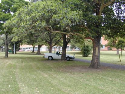
Figure 10 Vehicle running in the outdoor terrain. The video shows the different areas traversed by the vehicle including some sections taken from the laser viewpoint location.

 

Figure 11 presents the final navigation map and vehicle trajectory estimated by the system. A relative map was used to facilitate the de-correlation process. This map has a number of bases formed by two landmarks. The observations of the features closed to a base are obtained relative to this new coordinate system. The selection of the location of the bases is a function of the range of the external sensor. The coordinates of the bases are maintained in absolute form.

The accuracy of this map is determined by the initial vehicle position uncertainty and the quality of the combination of dead reckoning and external sensors.

Figure 11Final trajectory and navigation map. The intersection of the bases are presented with a ‘+’ and the other end of the segment with a ‘o’. The relative landmarks are represented with ‘*’ and its association with a base is represented with a line joining the landmark with the origin of the relative coordinate system. In this run 19 bases were created. The video presents the map building process.

Figure 12 presents the final estimation error of the features in the map. It can be seen that after 20 minutes the estimated error of all the features are below 70 cm. The video linked with this Figure is of fundamental importance to understand the behaviour of the SLAM algorithm. At the beginning of the experiment the system searches for features in the environment and creates new states with the location of the features that remain stable for a certain period of time. The evolution of the magnitude of the covariance of the elements of the state vector is shown in the video. Due to the correlations, new observations will reduce the magnitude of the error of all states except for the first three, which correspond to the position of the vehicle. The estimated errors of these three states grow when the vehicle explores new regions and decreases when the vehicle returns to known areas. The initial uncertainty of the new features will be function of the uncertainty of the vehicle states when first seen and the noise characteristic of the external sensor. These behaviours are clearly shown in the video and should be correlated to the path followed by the vehicle presented above. Finally the system ends the map building and localization process with a navigation map of 500 states.

Figure 12 Final estimated error of the 500 states. It can be seen that the maximum estimated error is below 0.7 meters. The video presents the evolution of these error when the vehicle is incorporating new features into the map.

Figure 13 shows a time evolution of standard deviation of few features. The dotted line corresponds to the compressed filter and the solid line to the full SLAM. It can be seen that the estimated error of some features are not continuously updated with the compressed filter. These features are not in the local area. Once the vehicle makes a transition the system updates all the features performing a full SLAM update. At this time the features outside the local area are updated in one iteration and the estimated error become exactly equal to the full SLAM. This is clearly shown in the video where enhanced views of the full and compressed SLAM algorithm are superimposed with different level of zooming. This demonstrates that while working in a local area it is not necessary to perform a full update considering all the feature of the map. The algorithm can update the local states at the frequency of the external sensor with reduced computational cost and then propagate the information gained in the local area to the rest of the states in the map without any loss of information.

Figure 13Features estimated position error for full Slam and compressed filter. The solid line shows the estimated error estimated with the full SLAM algorithm. This algorithm updates all the featuress with each observation. The dotted line shows the estimated error evaluated with the compressed filter. The landmark that are not in the local area are only updated when the vehicle leaves the local area.  At this time a full updates is performed and the estimated error becomes exactly equal to full SLAM.

Full SLAM implementation is required each time the system makes a transition to a new area. This work proposed a simplification based on neglecting the covariance update of states whose change in covariance is significant smaller than its actual covariance. The algorithm is still consistent since the cross-correlations are updated. The final result of map building and localization was compared with the full SLAM implementation and negligible differences were detected. They can only be appreciated by zooming into the picture to find errors of the order of less than 10 mm. This is shown in the video attached to the Figure.

Figure 14 Comparison between full SLAM and the compressed algorithm with the full updates using the simplification proposed.

7          Conclusion and future research.

This work presents real-time algorithms and implementation issues of Simultaneous Localization and Map Building (SLAM) with emphasis to outdoor land vehicle applications in large environments. The aspect of feature detection and validation is investigated to reliable detect the predominant features in the environment. The SLAM algorithm presented uses a compressed filter that reduce the standard SLAM computational requirement making possible the application of this algorithm in environments with more than 10000 landmarks. Algorithms to simplify the full update are also presented that results in a near optimal solution. Finally the algorithms are validated with experimental results obtained with a standard vehicle running in a completely unstructured outdoor environment. The results of this work are enhanced by the use of a series of multimedia facilities to demonstrate the problematic of outdoor navigation in unstructured environments. The raw time stamp dead-reckoning and laser data can also be accessed with the matlab code used to identify the features. This is essential to compare localization and map building results obtained with other localization algorithms.

Although the state of the art of sensors allows to perform SLAM in significant large environments at least four areas of research are of importance to extend these ranges:

High Frequency information: The incorporation of high frequency information increases the exploration range of the SLAM algorithms. This is also another important area of research. If no absolute position data become available the system will not be able to navigate for extended period of time in new areas without coming back to known areas.

Besides laser and radar scanners, investigation has gone into employing video cameras to provide addition information into SLAM applications. In a video image, a great deal of information is associated with objects that are within view, such as width, height, colour and texture [15]. Using current imaging techniques of edge and corner detection, features can be distinguished and identified in a single image frame. Inherently, 2D images cannot provide the distance information of these features; they do however return a bearing to the feature, relative to the camera.  Repeated observations and position estimates of the camera, then allow triangulation of the feature’s global position, which can then be used in the SLAM algorithm. This method is known as Bearing-Only SLAM

 

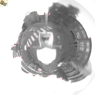
Figure 15  Point feature extraction and tracking from video information       ( Animated Gif)

 

To ensure triangulation for the initial estimation and further data associations of the features in subsequent image frames, the Kanade-Lucas-Tomasi (KLT) tracker can be used, [14]. The KLT tracker is an algorithm that finds the closest association of a selected pixel and its neighbours taken from one image within another image, and thus returning the feature’s position in the new image. This is used in this application on sequential images to provide the observation information of the feature, with a beginning estimate of the new pixel location retrieved from the SLAM algorithm.

To further the field of vision of the camera, we are also looking at the use of a panoramic camera. This is a normal video camera pointed at a hyperbolic mirror, which returns a warped 360° view of the environment. The use of this camera in Bearing-Only SLAM would increase the robustness of the algorithm, since normal cameras have a field of vision of only 30°. Investigation is now being done to apply corner detection and the KLT tracking algorithm to the panoramic image. Figure 15 and the Video linked to it shows an outdoor application of the KLT algorithm where it can be appreciated that the point features are consistently tracked during the run.

 

Robust Data Association: A key weakness of the Kalman filter based approach to SLAM is its dependence on correct association of observed features to mapped features. A miss-association results in an inconsistent reduction of estimated uncertainty while increasing the actual error. A single incorrect assignment may cause the filter to diverge (i.e., fail irretrievably). In situations with high feature clutter and large location uncertainties, it becomes necessary to devise a means of ensuring correct association. Although this problem has been addressed using the geometry of the environment [17], or using more complex data association methods [16] it still requires further research to add the robustness required for cluttered outdoor environments.

Closing a large loop. One of the problems of SLAM algorithms is known as closing large loops. If the vehicle has covered large areas before revisiting a known area then, depending on the quality of dead reckoning and external sensors the system will accumulate an error that will prevent correct data association when returning to a known area. The system will eventually see the old features but creates new states since due to the error accumulated during the exploration they will be outside the validation gate. This problem can be appreciated in Figure 16 . The system started at coordinate (0,0), performed a large loop and generated a slightly erroneous trajectory when back. Although some more sophisticated data association techniques can be used to detect this problem large updates may be required due to errors in the vehicle and sensor models. These large updates may violate some of the assumption of the Kalman Filter. Actual research is in progress to develop consistent algorithms to update the states corresponding to vehicle and landmarks once a large loop is closed.

Figure 16The system stated at coordinate (0,0), performed a large loop and when back generated an erroneous trajectory creating new states.

 

Information Maps. Once the vehicle has traversed a given area for a period of time, in addition to the navigation map, we can evaluate an information map as shown in Figure 17 . This map was built for a 2-D application. It gives the amount of information that can be gained if the vehicle is positioned in a particular place of the grid. As can be seen there are regions that have not been explored and are represented with zero information.  The regions with maximum information are the areas with enough number of features that have been incorporated into the map and known to have low error covariances. This map can be evaluated in real time with the available information with very low computational cost. Then the trajectory planner can use this information to obtain the best path to achieve different objectives such as explore new areas, reach a particular destination minimizing the localization errors, etc.

Figure 17Information map of the area. The areas with large number of features present large amount of information.

 

 

References

[1]     Elfes A., “Occupancy Grids: A probabilistic framework for robot perception and navigation”, Ph. D. Thesis, department of Electrical Engineering, Carnegie Mellon University, 1989.

[2]     Stentz A., Ollis M., Scheding S., Herman H., Fromme C., Pedersen J., Hegardorn T, McCall R., Bares J., Moore R., “Position Measurement for automated mining machinery”, Proc. of the International Conference on Field and Service Robotics, August 1999.

[3]     Durrant-Whyte Hugh F., "An Autonomous Guided Vehicle for Cargo Handling Applications". Int. Journal of Robotics Research, 15(5): 407-441, 1996.

[4]     Guivant J., Nebot E. and Durrant-Whyte H., "Simultaneous localization and map building using natural features in outdoor environments", IAS-6 Intelligent Autonomous Systems 25-28 July 2000, Italy, pp 581-586.

[5]     Leonard J. J. and Feder H. J. S., “A computationally efficient method for large-scale concurrent mapping and localization”, Ninth International Symposium on Robotics Research, pp 316-321, Utah, USA, October 1999.

[6]     Thrun S., Fox D., Bugard W., “Probabilistic Mapping of and Environment by a Mobile Robot”, Proc. Of 1998 IEEE, Belgium, pp 1546-1551.

[7]     Leonard J., Durrant-Whyte H., “Simultaneous map building and Localization for an autonomous mobile robot”, Proc. IEEE Int. Workshop on Intelligent Robots and systems, pp 1442-1447, Osaka , Japan.

 [8]    Williams SB, Newman P, Dissanayake MWMG, Rosenblatt J. and Durrant-Whyte HF "A decoupled, distributed AUV control architecture". 31st International Symposium on Robotics 14-17 May 2000, Montreal PQ, Canada. Proceedings of the 31st International Symposium on Robotics, vol 1, pp 246-251, Canadian Federation for Robotics Ottawa, ON, 1999. ISBN 0-9687044-0-9.

[9]     Guivant J., Nebot E., Baiker S., “Localization and map building using laser range sensors in outdoor applications”, Journal of Robotic Systems, Volume 17, Issue 10, 2000, pp 565-583

[10]   Sukkarieh S., Nebot E., Durrant-Whyte , “A High Integrity IMU/GPS Navigation Loop for Autonomous Land Vehicle applications”, IEEE Transaction on Robotics and Automation, June 1999, p 572-578.

[11]   Scheding, S. , Nebot E. M., and Durrant-Whyte H., “High integrity Navigation using frequency domain techniques”, IEEE Transaction of System Control Technology, July 2000, pp 676-694.

[12]   Motalier P., Chatila R., “Stochastic multi-sensory data fusion for mobile robot location and environmental modelling”, In Fifth Symposium on Robotics Research, Tokyo, 1989.

 [13]  Guivant J, Nebot E "Compressed Filter for Real Time Implementation of Simultaneous Localization and Map Building". To be published in Field and Service Robot 2001 June 2001, Finland.

 [14] Carlo Tomasi and Takeo Kanade. “Detection and Tracking of Point Features”. Carnegie Mellon University Technical Report CMU-CS-91-132, April 1991.

[15]   A.Mallet , S.Lacroix , L.Gallo, “Position estimation in outdoor environments using pixel tracking and stereovision”,  2000 IEEE International Conference on Robotics and Automation (ICRA'2000), San Francisco (USA), 24-28 Avril 2000, Vol.4, pp.3519-3524

 [16]  Neira J., Tardos J., “Robust and feasible data association for simultaneous localization and map building”, IEEE conference on Robotic and Automation, Workshop W4, San Francisco , USA, 2000.

[17] T. Bailey, E. Nebot, J. Rosemblat, H. Durrant Whyte, “Data Association for Mobile Robot Navigation: A Graph Theoretic Approach”, IEEE International Conference on Robotics and Automation, San Francisco, USA, April 2000, pp 2512-2517.